All the examples might not be up to date on the website, please go to our GitLab repository and download latest version of the notebook.

Simple dose computation and optimization on a real CT image

Author : Eliot Peeters

In this example we are going to see how to :

Import real dicom images and RT struct
Create a plan
Compute beamlets
Optimize a plan with beamlets
Save a plan and beamlets
Compute DVH histograms

import numpy as np
from matplotlib import pyplot as plt

#Import the needed opentps.core packages

from opentps.core.data.plan import PlanDesign
from opentps.core.data import DVH
from opentps.core.io import mcsquareIO
from opentps.core.io.scannerReader import readScanner
from opentps.core.processing.doseCalculation.doseCalculationConfig import DoseCalculationConfig
from opentps.core.processing.doseCalculation.mcsquareDoseCalculator import MCsquareDoseCalculator
from opentps.core.io.dataLoader import readData
from opentps.core.data.plan import ObjectivesList
from opentps.core.data.plan import FidObjective
from opentps.core.io.serializedObjectIO import saveBeamlets, saveRTPlan, loadBeamlets, loadRTPlan

In the next cell we configure the CT scan model used for the dose calculation and the bdl model. The ones used in this example are the default configuration of openTPS wich may lead to some imprecision.

ctCalibration = readScanner(DoseCalculationConfig().scannerFolder)
bdl = mcsquareIO.readBDL(DoseCalculationConfig().bdlFile)

Data importation

The dataset used in this example comes from the Proknow website, 2018 TROG Plan Study: SRS Brain. The readData functions automatically import the subfolders and detects the type of data (CT or RT_struct).

ctImagePath = "Data/ProKnows_2018_TROG_Plan_Study_SRS_Brain"
data = readData(ctImagePath)

rt_struct = data[0]
ct = data[1]

rt_struct.print_ROINames()

RT Struct UID: 2.16.840.1.114362.1.6.6.9.161209.11109530676.470491132.964.204
  [0]  GTV1-20Gy
  [1]  GTV2-20Gy
  [2]  GTV3-20Gy
  [3]  GTV4-20Gy
  [4]  Eye_L
  [5]  Eye_R
  [6]  Lens_L
  [7]  Lens_R
  [8]  OpticNerve_L
  [9]  OpticNerve_R
  [10]  Optic Chiasm
  [11]  Hippocampus_L
  [12]  Hippocampus_R
  [13]  Brainstem
  [14]  Brain
  [15]  BODY
  [16]  Bones
  [17]  Normal Brain
  [18]  GTV5-20Gy
  [19]  GTV-Total

For the purpose of the demonstration we are going to use only 3 different ROI. Note that it is important to specify the CT origin,gridSize and spacing to the getBinaryMask function in order to have a correct binary mask.

target_name = "GTV4-20Gy"
target = rt_struct.getContourByName(target_name).getBinaryMask(origin=ct.origin,gridSize=ct.gridSize,spacing=ct.spacing)

OAR_brain = rt_struct.getContourByName("Brain").getBinaryMask(origin=ct.origin,gridSize=ct.gridSize,spacing=ct.spacing)
OAR_brainstem = rt_struct.getContourByName("Brainstem").getBinaryMask(origin=ct.origin,gridSize=ct.gridSize,spacing=ct.spacing)
OAR_optic_chiasm = rt_struct.getContourByName("Optic Chiasm").getBinaryMask(origin=ct.origin,gridSize=ct.gridSize,spacing=ct.spacing)

For further plots we can extract the indexes of the centerOfMass of the tumor.

COM_coord = target.centerOfMass
COM_index = target.getVoxelIndexFromPosition(COM_coord)
Z_COORD = COM_index[2]

MCsquare configuration

We now initialize a MCsquareDoseCalculator and provide the beamModel and ctCalibration imported above.

# Configure MCsquare
mc2 = MCsquareDoseCalculator()
mc2.beamModel = bdl
mc2.ctCalibration = ctCalibration

Plan design

In the next section we create a planDesign object with 3 beams (of no medical relevance, we just use them for demonstration). There are multiple parameters which can affect computation time :

targetMargin : a higher margin will increase the time used to dilate the mask
spotSpacing : a lower spot spacing will result in more beamlets therefore longer beamlets calculation time
layerSpacing : a lower layer spacing will result in more beamlets therefore longer beamlets calculation time

# Design plan
beamNames = ["Beam1","Beam2","Beam3"]
gantryAngles = [0.,45.,315.]
couchAngles = [0.,0.,0.]

# Generate new plan
planDesign = PlanDesign()
planDesign.ct = ct
planDesign.gantryAngles = gantryAngles
planDesign.targetMask = target
planDesign.beamNames = beamNames
planDesign.couchAngles = couchAngles
planDesign.calibration = ctCalibration
planDesign.spotSpacing = 5.0
planDesign.layerSpacing = 5.0
planDesign.targetMargin = 5.0

plan = planDesign.buildPlan()  # Spot placement
plan.PlanName = "NewPlan"

08/08/2023 09:33:47 AM - opentps.core.data.plan._planDesign - INFO - Building plan ...
08/08/2023 09:33:49 AM - opentps.core.processing.planOptimization.planInitializer - INFO - Target is dilated using a margin of 5.0 mm. This process might take some time.
08/08/2023 09:33:49 AM - opentps.core.processing.imageProcessing.roiMasksProcessing - INFO - Using SITK to dilate mask.
08/08/2023 09:34:32 AM - opentps.core.data.plan._planDesign - INFO - New plan created in 44.99794363975525 sec
08/08/2023 09:34:32 AM - opentps.core.data.plan._planDesign - INFO - Number of spots: 609

Beamlets computation and initial dose computation

In the next section we compute the beamlets (this is the most computer-intensive part). We have set the numbers of protons to 5e4.

mc2.nbPrimaries = 5e4
beamlets = mc2.computeBeamlets(ct, plan)
plan.planDesign.beamlets = beamlets

After the beamlets computation we can save the plan and the beamlets to reuse them in the future.

WARNING : the saveRTPlan function automatically remove the beamlets from the memory, if you want to save the beamlets, you have to call the saveBeamlets function before. Those files can be heavy !

Afterward you can load the plan and the beamlets via the loadRTPlan and loadBeamlets functions.

# Save the plan and the beamlets
saveBeamlets(beamlets,"Data/SimpleRealDoseComputationOptimization_beamlets.blm")
saveRTPlan(plan,"Data/SimpleRealDoseComputationOptimization_plan.tps")
plan = loadRTPlan("Data/SimpleRealDoseComputationOptimization_plan.tps")
plan.planDesign.beamlets = loadBeamlets("Data/SimpleRealDoseComputationOptimization_beamlets.blm")

Note that in the next cell we have augmented the number of protons for the dose computation (computeDose) to have a more accurate dose. This dose is computed with all the weights of the beamlets set to 1.

mc2.nbPrimaries = 1e7
dose_before_opti = mc2.computeDose(ct,plan)

Plan optimization

We will now optimize the plan with and without OAR to compare the differences. We first create an ObjectivesList and then add objectives via the addFidObjective which can be either DMIN, DMAX or DMEAN. Note that you can also create other objectives and implement them via the addExoticObjective fucntion.

plan.planDesign.objectives = ObjectivesList() #create a new objective set
plan.planDesign.objectives.setTarget(target.name, 20.0) #setting a target of 20 Gy for the target
plan.planDesign.objectives.fidObjList = []
plan.planDesign.objectives.addFidObjective(target, FidObjective.Metrics.DMAX, 19.5, 1.0)
plan.planDesign.objectives.addFidObjective(target, FidObjective.Metrics.DMIN, 20.5, 1.0)
plan.planDesign.defineTargetMaskAndPrescription()

We will use the Scipy-LBFGS as solver for this example but other are also implemented such as :

Scipy-BFGS
Scipy-LBFGS
Gradient
BFGS
LBFGS
FISTA
LP

Feel also free to specify a maxit to the IMPTPlanOptimizer object to speed up the program.

from opentps.core.processing.planOptimization.planOptimization import IMPTPlanOptimizer

solver = IMPTPlanOptimizer(method='Scipy-LBFGS',plan=plan)
w, doseImage, ps = solver.optimize()
plan.spotMUs = np.square(w).astype(np.float32)

We can now recompute the dose.

doseImage_opti = mc2.computeDose(ct,plan)

We here reload the plan in order to reset all weights and the filtering (after optimization, spots that are bellow the solver.thresholdSpotRemoval and corresponding weights are removed).

plan = loadRTPlan("Data/SimpleRealDoseComputationOptimization_plan.tps")
plan.planDesign.beamlets = loadBeamlets("Data/SimpleRealDoseComputationOptimization_beamlets.blm")
plan.planDesign.objectives = ObjectivesList() #create a new objective set
plan.planDesign.objectives.setTarget(target.name, 20.0) #setting a target of 20 Gy for the target
plan.planDesign.objectives.fidObjList = []
plan.planDesign.objectives.addFidObjective(target, FidObjective.Metrics.DMAX, 20.5, 1.0)
plan.planDesign.objectives.addFidObjective(target, FidObjective.Metrics.DMIN, 19.5, 1.0)
plan.planDesign.objectives.addFidObjective(OAR_brain, FidObjective.Metrics.DMAX, 8.0, 1.0)
plan.planDesign.objectives.addFidObjective(OAR_brainstem, FidObjective.Metrics.DMAX, 5.0, 1.0)
plan.planDesign.objectives.addFidObjective(OAR_optic_chiasm, FidObjective.Metrics.DMAX, 2.0, 1.0)
plan.planDesign.defineTargetMaskAndPrescription()

solver = IMPTPlanOptimizer(method='Scipy-LBFGS',plan=plan)
w, doseImage, ps = solver.optimize()
plan.spotMUs = np.square(w).astype(np.float32)

doseImage_opti_OAR = mc2.computeDose(ct,plan)

DVH histograms

We can create simple DVH plots with the DVH objects. Take a look at the class properties to find the D95, …

target_DVH = DVH(target,doseImage_opti_OAR)
target_DVH_No_OAR = DVH(target,doseImage_opti)
brain_DVH = DVH(OAR_brain,doseImage_opti_OAR)
brainstem_DVH = DVH(OAR_brainstem,doseImage_opti_OAR)
optic_chiasm_DVH = DVH(OAR_optic_chiasm,doseImage_opti_OAR)

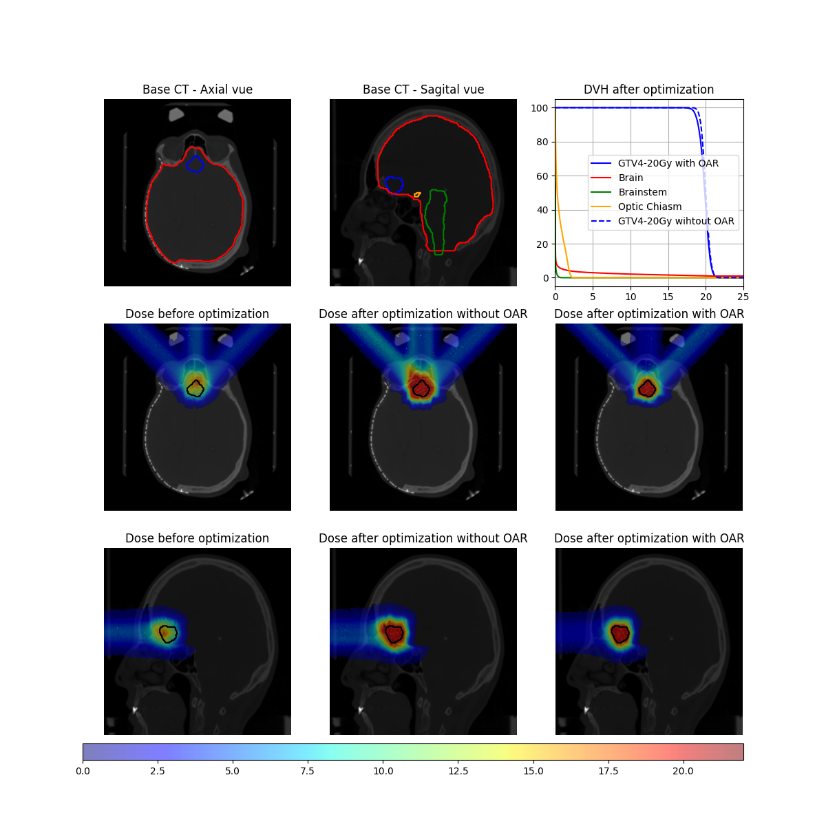
Final plots

Now that the different optimizations are done, we can display the results.

from skimage.transform import resize
image_ct_axial = ct.imageArray[:,:,Z_COORD].transpose(1,0)
image_target_axial = target.imageArray[:,:,Z_COORD].transpose(1,0)
image_brain_axial = OAR_brain.imageArray[:,:,Z_COORD].transpose(1,0)
image_brainstem_axial = OAR_brainstem.imageArray[:,:,Z_COORD].transpose(1,0)
image_optic_chiasm_axial = OAR_optic_chiasm.imageArray[:,:,Z_COORD].transpose(1,0)
image_dose_before_opti_axial = dose_before_opti.imageArray[:,:,Z_COORD].transpose(1,0)
image_dose_opti_axial = doseImage_opti.imageArray[:,:,Z_COORD].transpose(1,0)
image_dose_opti_OAR_axial = doseImage_opti_OAR.imageArray[:,:,Z_COORD].transpose(1,0)

image_ct_sagital = resize(np.rot90(ct.imageArray[COM_index[0],:,:]),(ct.gridSize[:-1]))
image_target_sagital = resize(np.rot90(target.imageArray[COM_index[0],:,:]),(ct.gridSize[:-1]))
image_brain_sagital = resize(np.rot90(OAR_brain.imageArray[COM_index[0],:,:]),(ct.gridSize[:-1]))
image_brainstem_sagital = resize(np.rot90(OAR_brainstem.imageArray[COM_index[0],:,:]),(ct.gridSize[:-1]))
image_optic_chiasm_sagital = resize(np.rot90(OAR_optic_chiasm.imageArray[COM_index[0],:,:]),(ct.gridSize[:-1]))
image_dose_before_opti_sagital = resize(np.rot90(dose_before_opti.imageArray[COM_index[0],:,:]),(ct.gridSize[:-1]))
image_dose_opti_sagital = resize(np.rot90(doseImage_opti.imageArray[COM_index[0],:,:]),(ct.gridSize[:-1]))
image_dose_opti_OAR_sagital = resize(np.rot90(doseImage_opti_OAR.imageArray[COM_index[0],:,:]),(ct.gridSize[:-1]))

min_dose_val = 0.1
image_dose_before_opti_axial[image_dose_before_opti_axial <= min_dose_val] = np.nan
image_dose_opti_axial[image_dose_opti_axial <= min_dose_val] = np.nan
image_dose_opti_OAR_axial[image_dose_opti_OAR_axial <= min_dose_val] = np.nan
image_dose_before_opti_sagital[image_dose_before_opti_sagital <= min_dose_val] = np.nan
image_dose_opti_sagital[image_dose_opti_sagital <= min_dose_val] = np.nan
image_dose_opti_OAR_sagital[image_dose_opti_OAR_sagital <= min_dose_val] = np.nan

vmin=0
vmax=22

fig, ax = plt.subplots(3,3,figsize=(12,12))

ax[0,0].imshow(image_ct_axial,cmap="gray")
ax[0,0].contour(image_target_axial,colors="blue")
ax[0,0].contour(image_brain_axial,colors="red")
ax[0,0].contour(image_brainstem_axial,colors="green")
ax[0,0].contour(image_optic_chiasm_axial,colors="orange")
ax[0,0].axis("off")
ax[0,0].set_title("Base CT - Axial vue")

ax[0,1].imshow(image_ct_sagital,cmap="gray")
ax[0,1].contour(image_target_sagital,colors="blue")
ax[0,1].contour(image_brain_sagital,colors="red")
ax[0,1].contour(image_brainstem_sagital,colors="green")
ax[0,1].contour(image_optic_chiasm_sagital,colors="orange")
ax[0,1].axis("off")
ax[0,1].set_title("Base CT - Sagital vue")

ax[0,2].plot(target_DVH.histogram[0],target_DVH.histogram[1],label=target_DVH.name + " with OAR",color="blue")
ax[0,2].plot(brain_DVH.histogram[0],brain_DVH.histogram[1],label=brain_DVH.name, color="red")
ax[0,2].plot(brainstem_DVH.histogram[0],brainstem_DVH.histogram[1],label=brainstem_DVH.name, color="green")
ax[0,2].plot(optic_chiasm_DVH.histogram[0],optic_chiasm_DVH.histogram[1],label=optic_chiasm_DVH.name, color="orange")
ax[0,2].plot(target_DVH_No_OAR.histogram[0],target_DVH_No_OAR.histogram[1],label=target_DVH.name + " wihtout OAR",color="blue",linestyle="dashed")
ax[0,2].set_xlim(0,25)
ax[0,2].grid(True)
ax[0,2].legend()
ax[0,2].set_title("DVH after optimization")

ax[1,0].imshow(image_ct_axial,cmap="gray")
dose_bar_ref = ax[1,0].imshow(image_dose_before_opti_axial,cmap="jet",alpha=.5,vmin=vmin,vmax=vmax)
ax[1,0].contour(image_target_axial,colors="black")
ax[1,0].set_title("Dose before optimization")
ax[1,0].axis("off")

ax[1,1].imshow(image_ct_axial,cmap="gray")
ax[1,1].imshow(image_dose_opti_axial,cmap="jet",alpha=.5,vmin=vmin,vmax=vmax)
ax[1,1].contour(image_target_axial,colors="black")
ax[1,1].set_title("Dose after optimization without OAR")
ax[1,1].axis("off")

ax[1,2].imshow(image_ct_axial,cmap="gray")
ax[1,2].imshow(image_dose_opti_OAR_axial,cmap="jet",alpha=.5,vmin=vmin,vmax=vmax)
ax[1,2].contour(image_target_axial,colors="black")
ax[1,2].set_title("Dose after optimization with OAR")
ax[1,2].axis("off")

ax[2,0].imshow(image_ct_sagital,cmap="gray")
ax[2,0].imshow(image_dose_before_opti_sagital,cmap="jet",alpha=.5,vmin=vmin,vmax=vmax)
ax[2,0].contour(image_target_sagital,colors="black")
ax[2,0].set_title("Dose before optimization")
ax[2,0].axis("off")

ax[2,1].imshow(image_ct_sagital,cmap="gray")
ax[2,1].imshow(image_dose_opti_sagital,cmap="jet",alpha=.5,vmin=vmin,vmax=vmax)
ax[2,1].contour(image_target_sagital,colors="black")
ax[2,1].set_title("Dose after optimization without OAR")
ax[2,1].axis("off")

ax[2,2].imshow(image_ct_sagital,cmap="gray")
ax[2,2].imshow(image_dose_opti_OAR_sagital,cmap="jet",alpha=.5,vmin=vmin,vmax=vmax)
ax[2,2].contour(image_target_sagital,colors="black")
ax[2,2].set_title("Dose after optimization with OAR")
ax[2,2].axis("off")
cb_ax = fig.add_axes([0.1, 0.08, 0.8, 0.02])
fig.colorbar(dose_bar_ref,cax=cb_ax,location="bottom")
plt.savefig("img/SimpleRealDoseComputationOptimization_output.png")
plt.close()

png

Download this notebook via our GitLab repository